Market Regime Detection & Regime-Conditional Factor Rotation:
Market returns are not generated by a single, stationary process — they pass through distinct regimes: a calm trending bull, a high-volatility bear, a choppy transition. Those regimes are not directly observable, but they leave a fingerprint in the joint sequence of returns and volatility, and — crucially — the factor premia themselves change sign across them (momentum pays in bull markets and reverses in bear markets; value and quality come into their own when volatility spikes). This project operationalises that idea end to end. A 3-state Gaussian Hidden Markov Model, fit by Baum–Welch EM on a low-dimensional (market return, realised volatility) observation, infers the latent regime; the states are relabelled economically (calm → volatile) and validated against known crisis windows. A separate gradient-boosted alpha model (XGBoost, with a scikit-learn fallback) is then trained per regime on the cross-section of factor exposures, and their predictions are blended by the current causal regime posterior — a soft, posterior-weighted rotation rather than hard switching. The decisive test is honest and out-of-sample: a strict walk-forward comparison of the regime-blended signal against a single unconditional model and a static factor floor, scored by information coefficient and long–short Sharpe, net of turnover cost, with a permutation significance check. A focused Markov-Switching VAR module extends the idea to joint equity/bond dynamics as a macro overlay. This is a full modernisation of a 2020 academic assignment (HMM + One-Class SVM bull/bear detection on the iShares MSCI EAFE ETF), whose original paper is preserved at the bottom of this page. Built on Python 3.11+ with hmmlearn, xgboost, scikit-learn, numpy, scipy, pandas, plotly, streamlit, pydantic v2 and typer; packaged with hatchling and tested with pytest against deterministic seed-42 fixtures.
I. Interactive Dashboard:
The dashboard below runs entirely in the browser via stlite (Streamlit on WebAssembly — no server). XGBoost cannot run in Pyodide, so the in-browser demo fits a pure-NumPy Gaussian HMM (the same Baum–Welch EM the package uses) and blends per-regime ridge regressions by the causal posterior — it shows the identical pipeline (regime inference, posterior-blended factor rotation, and the cost-aware walk-forward comparison) instantly. The full project trains gradient-boosted trees. First load downloads Pyodide and may take 20–40 seconds.
II. Project Layout:
hmm_svm/  (package: regime_rotation)
├── pyproject.toml                              # Build config, deps, ruff + pytest settings
├── .env.example                                # REGIME_ETF / Fama-French (optional)
├── dashboard.html                              # Self-contained stlite browser demo (numpy HMM stand-in)
├── scripts/
│   └── make_thumbnail.py                       # Real matplotlib thumbnail (regime-coloured equity)
├── src/regime_rotation/
│   ├── data/
│   │   ├── synthetic.py                        # Regime-switching market simulator (premia flip per regime)
│   │   ├── schemas.py                          # Pydantic v2 config / stats records
│   │   └── fetchers.py                         # yfinance ETF + Fama-French (optional)
│   ├── regimes/
│   │   ├── gaussian_hmm.py                     # Baum-Welch EM + forward-backward + Viterbi (pure numpy)
│   │   ├── labeler.py                          # Economic state labelling; CAUSAL filtered posteriors
│   │   └── ms_var.py                           # Markov-Switching VAR macro overlay
│   ├── models/
│   │   └── alpha.py                            # Unconditional vs per-regime GBM blend vs static floor
│   ├── eval/
│   │   ├── metrics.py                          # Rank IC, Sharpe, turnover, permutation p-value
│   │   └── backtest.py                         # Walk-forward (causal); gross + net of cost
│   ├── report/plots.py                         # Plotly: regime ribbon, IC bars, premium heatmap
│   ├── cli.py                                  # Typer CLI: regimes | compare | costs | regimeic | msvar | stats
│   └── app.py                                  # Streamlit server-side dashboard
└── tests/                                      # Seed-42 fixtures; HMM, causal posteriors, walk-forward, MS-VAR
III. The Latent-Regime Market (data/synthetic.py):
The simulator is governed by a latent Markov chain \(s_t \in \{0,1,2\}\) with a sticky transition matrix, so regimes persist for weeks. Each day the cross-section of asset returns is generated by
where \(m_t\) is the regime-dependent market return, \(z_{f,i,t-1}\) are three strictly-lagged, cross-sectionally standardised factor exposures (momentum, value, quality) known at the start of day \(t\), and \(\pi_{f,s}\) is the per-regime factor premium. The structural fact the whole project hinges on: \(\pi_{f,s}\) flips sign with the regime — momentum earns \(+0.0020\) in the bull state and \(-0.0018\) in the bear state. The HMM observes only the 2-vector \((m_t,\ \widehat{\sigma}_t)\) of market return and trailing realised volatility — exactly the parsimonious signal used to label regimes in practice.
IV. The Gaussian HMM (regimes/gaussian_hmm.py):
A self-contained multivariate-Gaussian HMM is implemented from scratch so the same algorithm runs in the package, the tests, and the browser (where hmmlearn cannot). The three classical problems are solved: a numerically-stable, log-domain forward–backward pass for the smoothed posteriors \(\gamma_{t,s}=P(s_t=s\mid y_{1:T})\) and log-likelihood; Baum–Welch EM for the parameters \((\pi_0, A, \mu_s, \Sigma_s)\); and Viterbi for the most-likely path. Raw HMM state indices are arbitrary, so states are relabelled by emission volatility (calm → volatile) for stable economic names. The hmmlearn backend is available as a cross-check and returns the identical interface.
def fit(self, X):                                # Baum-Welch EM
    self._init(X)                                # k-means++ seeding of the means
    for _ in range(self.n_iter):
        logB = self._log_emission(X)             # log N(x_t; mu_s, Sigma_s)
        loglik, gamma, xi = self._forward_backward(logB)   # E-step (log-domain, stable)
        self.loglik_history_.append(loglik)      # monotone non-decreasing (tested)
        # M-step: re-estimate start probs, transition matrix, per-state mean + covariance
        self.params.transmat = xi / xi.sum(1, keepdims=True)
        for s in range(self.n_states):
            w = gamma[:, s]
            self.params.means[s]  = (w[:, None] * X).sum(0) / w.sum()
            self.params.covars[s] = weighted_covariance(X, self.params.means[s], w)
V. Causal Posteriors & the No-Leak Backtest (regimes/labeler.py, eval/backtest.py):
The single most important methodological point. A walk-forward backtest must never let a day-\(t\) decision use the smoothed posterior \(\gamma_{t,s}\), because smoothing conditions on the future \(y_{t+1:T}\). Instead we use the filtered posterior \(P(s_t\mid y_{1:t})\), computed from the forward recursion alone, so the regime belief at \(t\) sees only data up to \(t\). The HMM and the per-regime alpha models are refit on each expanding training window; every test day is predicted exactly once and is strictly later than its training set; and returns at \(t\) are predicted from exposures known at \(t-1\). A test asserts the prefix-invariance of the filtered posterior — appending future data must not change the belief at an earlier day.
def test_filtered_posterior_prefix_invariance(fitted, panel):
    obs = panel.observations()
    t = 500
    short = filtered_posteriors(fitted.model, obs[:t+1], fitted.order)[t]
    full  = filtered_posteriors(fitted.model, obs,        fitted.order)[t]
    assert np.allclose(short, full, atol=1e-8)     # day-t belief never sees the future
VI. Regime-Conditional Factor Rotation (models/alpha.py):
Three models are compared head to head, all strictly causal. The unconditional model is one gradient-boosted regressor on the pooled cross-section — the strong, simple baseline that does not know the regime. The regime-blend trains a separate gradient-boosted regressor per regime and blends their predictions by the current causal posterior, \(\hat{\alpha}_{i,t} = \sum_s P(s_t=s\mid y_{1:t})\, g_s(z_{i,t-1})\). The static factor model is a fixed equal-weight tilt — a regime-blind floor. Predictions are turned into a dollar-neutral, unit-gross long–short portfolio, and the realised cost is charged on the daily turnover.
VII. The Honest Result (cli.py compare):
Walk-forward out-of-sample over five expanding folds (\(n = 3{,}000\) days, 12 assets, 10 bps cost). The permutation \(p\)-value is a sign-flip test on the daily IC series — it separates real signal from lucky noise.
| Model | IC | IC IR | IC p-val | Sharpe gross | Sharpe NET | Turnover |
|---|---|---|---|---|---|---|
| Static factor (floor) | +0.076 | +9.8 | 0.001 | +4.38 | +3.45 | 0.261 |
| Unconditional (baseline) | +0.083 | +10.7 | 0.001 | +4.56 | +3.15 | 0.422 |
| Regime blend | +0.102 | +12.7 | 0.001 | +5.67 | +4.05 | 0.496 |
Honestly reported: the regime blend has a real, statistically significant edge — it lifts the information coefficient by \(+0.019\) over the unconditional model (\(p = 0.001\)) and the net Sharpe by \(+0.90\) — because it genuinely exploits the regime-dependent factor premia. But it is not a free lunch. It rotates exposure as the posterior shifts, so it turns over more (0.50 vs 0.42), and that is precisely the cost it must pay for the edge.
VIII. Where the Edge Erodes (cli.py costs):
The candid punchline. Because regime switching is turnover-hungry, its advantage is entirely contingent on cheap execution and shrinks monotonically as the cost of trading rises:
| Cost (bps) | Regime-blend NET Sharpe | Unconditional NET Sharpe | Edge |
|---|---|---|---|
| 0 | +5.67 | +4.56 | +1.12 |
| 10 | +4.05 | +3.15 | +0.90 |
| 30 | +0.83 | +0.33 | +0.51 |
| 50 | −2.29 | −2.45 | +0.16 |
At 50 bps both strategies lose money and the regime edge has all but vanished. The precise reframing: regime conditioning adds genuine value, but its worth is a function of trading cost. It is the right tool for a low-cost, patient allocator rotating factor sleeves; it is the wrong tool for a high-turnover book paying a wide spread. That contingency — not a headline Sharpe — is the deliverable.
IX. Per-Regime Attribution (cli.py regimeic):
Conditioning the out-of-sample IC on the causal regime shows where the blend earns its edge. The unconditional model is weakest in the calm bull state (where its pooled fit dilutes the strong momentum premium); the regime blend recovers exactly there, and adds further in the high-vol bear state where the momentum premium has reversed sign:
| Regime | Unconditional IC | Regime-blend IC |
|---|---|---|
| Low-vol bull | +0.048 | +0.072 |
| Transition | +0.114 | +0.114 |
| High-vol bear | +0.116 | +0.145 |
The HMM is also economically plausible: after relabelling, the calm state maps onto the true low-vol bull regime and the volatile state onto the true high-vol bear regime (recall \(> 0.5\) on both clean states); the transition regime is, fairly, the hardest to pin down, mirroring the genuine ambiguity of turning points.
X. Markov-Switching VAR Macro Overlay (regimes/ms_var.py):
A focused extension lifts the idea to joint dynamics. A Markov-Switching VAR(1), \(y_t = c_{s_t} + A_{s_t}\, y_{t-1} + \varepsilon_t\) with \(\varepsilon_t \sim \mathcal{N}(0,\Sigma_{s_t})\) and \(y_t = (\text{equity},\,\text{bond})\), is fit by an EM that is Baum–Welch with per-state conditional-Gaussian (VAR) emissions. Without being told, it recovers a calm, positive equity/bond-correlation regime and a flight-to-quality regime where the correlation flips negative — the textbook risk-off state in which bonds rally as equities fall:
| Regime | Frequency | Equity/bond correlation | Equity ann. vol |
|---|---|---|---|
| Calm | 62% | +0.25 | 0.143 |
| Flight-to-quality | 38% | −0.86 | 0.305 |
XI. CLI — cli.py:
# Install
pip install -e ".[dev]"

# Fit the HMM and print economically-labelled regimes
regime regimes

# The headline honest table: regime-blend vs unconditional vs static (gross + NET)
regime compare

# Sweep the transaction cost and watch the regime edge erode
regime costs

# Per-regime IC attribution
regime regimeic

# Markov-Switching VAR macro overlay (equity/bond flight-to-quality regime)
regime msvar

# Launch the server-side Streamlit dashboard
streamlit run src/regime_rotation/app.py
| Command | Key options | Output |
|---|---|---|
regime compare | --n, --states, --folds, --cost, --backend | Walk-forward IC / Sharpe (gross & net) leaderboard + p-value |
regime costs | --n, --folds | Net-Sharpe edge of the blend across a cost sweep |
XII. Test Suite:
Thirty-five tests, fully offline, seed-42. The substantive guarantees are tested, not just shapes: the HMM log-likelihood is monotone non-decreasing under Baum–Welch; the economic labelling sorts states calm → volatile; the filtered posterior is prefix-invariant (causal) and genuinely differs from the smoothed posterior; the walk-forward indices are out-of-sample and each test day is predicted exactly once; the regime blend beats the unconditional baseline on IC with significant signal; costs cannot increase Sharpe; the long–short weights are dollar-neutral and unit-gross; the permutation test detects a planted signal and rejects pure noise; and the Markov-Switching VAR recovers two distinct equity/bond correlation regimes.
def test_each_test_day_predicted_once(wf):
    assert len(wf.test_days) == len(np.unique(wf.test_days))   # no fold overlap

def test_regime_blend_beats_unconditional_ic(wf):
    assert wf.results["regime_blend"].ic_mean > wf.results["unconditional"].ic_mean

def test_models_have_significant_signal(wf):
    assert wf.results["regime_blend"].ic_pvalue < 0.05         # real signal, not noise
XIII. Configuration & Setup:
cd assets/projects/hmm_svm
python -m venv .venv && .venv\Scripts\Activate.ps1        # Windows
pip install -e ".[dev]"
regime compare                                            # reproduce the honest leaderboard
regime costs                                              # where the regime edge erodes
pytest -q                                                 # 35 tests, offline
streamlit run src/regime_rotation/app.py
No data download is required: the HMM, the alpha models, the tests and the dashboard all run on the synthetic regime-switching simulator with no API keys. The optional data/fetchers.py supports a real iShares MSCI EAFE (EFA) ETF series and the Fama–French factor returns for a real-data study.
Team:
Theodosios Dimitrasopoulos, personal project (a modernisation of an FE 690 assignment at the Stevens Institute of Technology).
Tools & methods:
Python 3.11, hmmlearn, XGBoost (scikit-learn fallback), scikit-learn, NumPy, SciPy, pandas, Pydantic v2, Typer, rich, Plotly, Streamlit, pytest, ruff, hatchling. Methods: Gaussian Hidden Markov Models (Baum–Welch EM, forward–backward, Viterbi); economic state labelling; causal filtered posteriors vs smoothing; regime-conditional gradient-boosted cross-sectional alpha with posterior-weighted blending; leak-free walk-forward (rolling-origin) validation; rank information coefficient, long–short Sharpe and turnover; sign-flip permutation significance testing; transaction-cost-aware evaluation; Markov-Switching VAR for joint equity/bond regime dynamics.
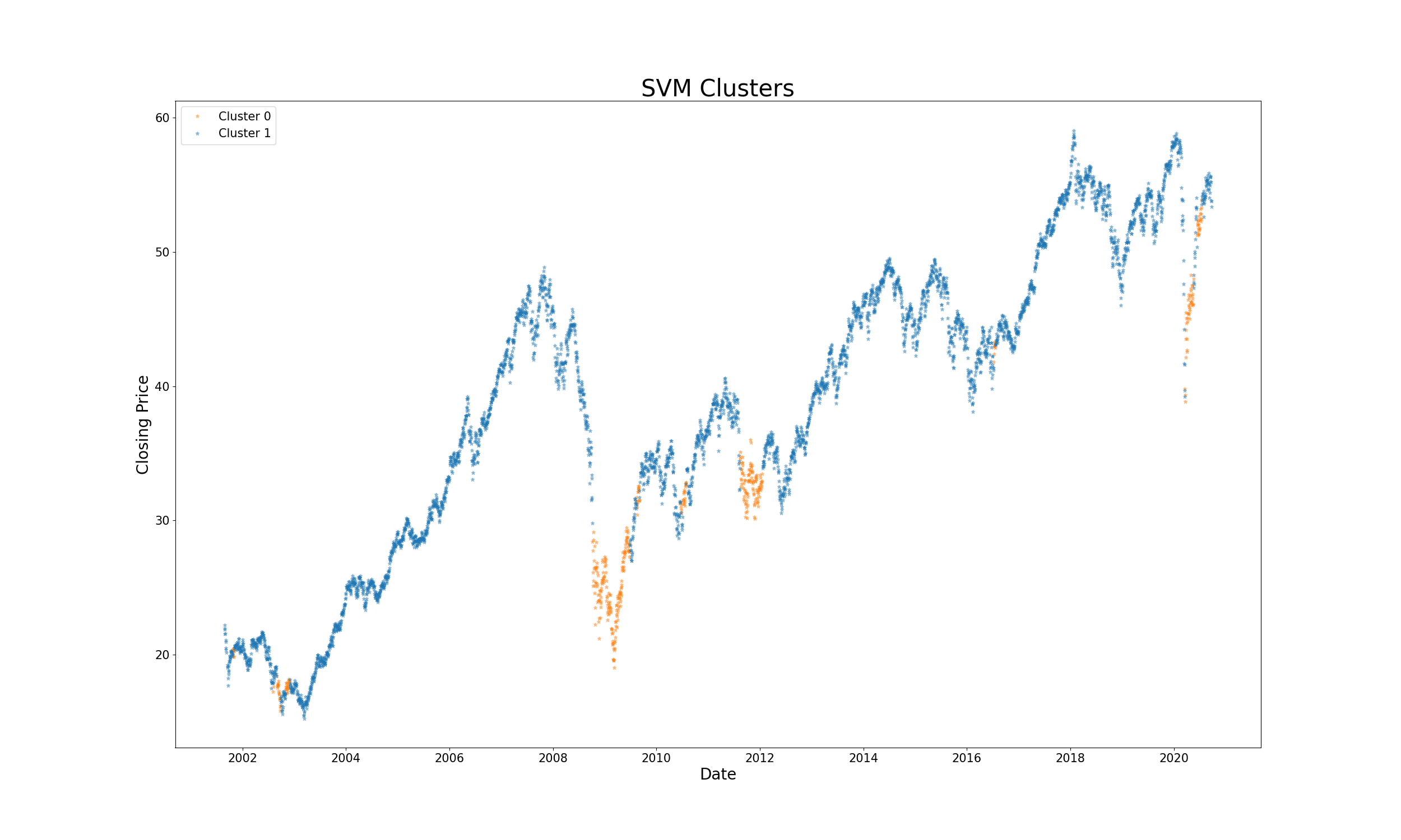
XIV. Original Academic Paper (2020):
This project began as a graduate assignment for FE 690: Machine Learning in Finance. The original study used a two-state Gaussian HMM and a One-Class SVM (with an RBF kernel, tuning \(\nu\) and \(\gamma\)) to detect bull/bear regimes in the iShares MSCI EAFE ETF (ticker EFA) from 2000–2020, motivated by using overnight international price action to inform a US market-on-open order. The figures and full report below are preserved unchanged; the work above generalises and modernises it — multi-state regimes, posterior-blended factor rotation, leak-free walk-forward validation, a transaction-cost honesty test, and a Markov-Switching VAR overlay (several of the “next steps” flagged in the original paper).

DOCUMENTS
The Github repository can be found here.
All requests for copies of the research, please forward to my university email address listed on my homepage.